Lab 2 - Motion In 2D
Table of Contents
In this lab, you will use the Kinematic Equations to first measure, and then predict, projectile motion. In the first experiment, you will launch a ball horizontally and make the necessary measurements to calculate the initial velocity of the projectile. In the second part, you will incline the launcher and use your results to predict the new range of the projectile.
\[ x_f = x_i + v_i \, t + \frac12 a\, t^2\] \[ v_f = v_i + a \, t\] \[ v_f^2 = v_i^2 +2\, a (x_f - x_i)\]
1. Experiment 1: Horizontal Shot
- Clamp the Ballistic Pendulum to the edge of a sturdy table. Make sure that the launcher is firing as close as possible to horizontal (make a note of this systematic error. ask the instructor if you are confused).
- Locate a clear line of fire at least 3 meters free of other classmates and other objects. Fire a test shot to observe the approximate range of the launcher.
Place a piece of white paper on the floor at the approximate impact point. Tape the white paper to the floor to make sure it does not move.
This lab includes error analysis. Please take care in the next step:
- After you are satisfied with the setup, start taking real notes on the experiment. Please recall from Lab 1,the goal at the end of lab is to have these 4 parts written on paper:
- Name, Lab, Date
- Sketch of the experimental setup with detailed dimensions
- Measurements corresponding to the sketch (include error estimates)
- Basic calculated result (without error propagation)
- Measure the initial height of the ball from the floor in meters. Take a moment to think where on the ball you should take this measurement to find the overall change in height. Also include your estimated error (standard deviation).
- Fire the launcher many times. You will be estimating the uncertainty of the range with statistics, so try to make a grouping of impacts. Record the horizontal range of each launch as a list on your lab records. (Around 10 launches seems appropriate here, but remember we are looking for statistical significance, so instructions indicating a “tight grouping” may be more informative than a launch count)
- Use the mean (average) to find your measured value of \(x_f\) and the standard deviation to find the error \(E[x_f]\).
- Use your knowledge of kinematics to calculate the velocity which the ball exits the launcher.
| \(x_i=\hspace{50mm}\) | \(y_i=\hspace{50mm}\) |
| \(x_f=\) | \(y_f=\) |
| \(v_{ix}=\) | \(v_{iy}=\) |
| \(v_{fx}=\) | \(v_{fy}=\) |
| \(a_x=\) | \(a_y=\) |
| \(\hspace{30mm}t=\) |
Checkpoint:
- records of height \(y\) (with error) and range \(x_f\) (with error)
- calculation of the initial velocity \(\vec{v}_i = (v_{ix}, v_{iy})\) using the kinematic equations
2. Experiment 2: Inclined Shot
Now you will incline the launcher, which will increase the range of the launcher.
- Loosen the bolts on the launcher and reposition the launcher to an incline between \(15^\circ\) and \(25^\circ\).
Use a meter stick to make an accurate measurement of the angle which you have set. To accomplish this, place a meter stick along the upper edge of the launcher to form the hypotenuse of a right triangle. Then use trig to estimate the angle to 3 digits of precision.
\(\theta\) =
Set up the launcher on the edge of the table and measure the new height (this height changes from part 1).
\(y\) =
- As is often the case, finding the spread of outcomes via error analysis is not easy (see below). Instead lets take a shortcut, and use the upper and lower estimates of velocity to predict the minimum and maximum range.
Use your knowledge of kinematics to calculate the minimum and maximum range using the upper and lower bound for velocity found in part 1:
| \(x_i=\hspace{50mm}\) | \(y_i=\hspace{50mm}\) |
| \(x_f=\) | \(y_f=\) |
| \(v_{ix}=\) | \(v_{iy}=\) |
| \(v_{fx}=\) | \(v_{fy}=\) |
| \(a_x=\) | \(a_y=\) |
| \(\hspace{30mm}t=\) |
\(x_{Max}\) = \(x_{Min}\) =
Checkpoint:
- Calculate the theoretical range of the shot using your average
- Measure a sample shot to verify your results agree with experiment
- Make sure you are comfortable with this before Exam 1
3. Part 3: Analysis of Error
Error propagation for Horizontal Shot
- Write down each algebraic equation you used calculate these results. First write an algebraic expression for \(t\), then write one for \(v_{ix}\). You will use these equations to propagate error. \[t(y) = \qquad\qquad\qquad v_{ix}(x_f,t)=\]
Use the error propagation formula to find the propagated error in time
\[E[t] = \sqrt{\left( \frac{\partial t}{\partial y} \cdot E[y] \right)^2 } = \frac{\partial t}{\partial y} \cdot E[y]\]
Use the error propagation formula to find the propagated error in velocity
\[E[v_{ix}] = \sqrt{\left( \frac{\partial v_{ix}}{\partial t} \cdot E[t] \right)^2 + \left( \frac{\partial v_{ix}}{\partial x_f} \cdot E[x_f] \right)^2 }\]
Checkpoint:
- Complete the derivation of error formulae for time and velocity
- Propagate error in velocity \(E[v_{ix}]\)
Error propagation for Inclined Shot (a dead end)
Propagating error leads to complications even in simple cases, such as kinematics. If you attempt to go headlong into the math, you arrive at the following: (This includes a clever substitute-eliminate trick)
Process to solve for range in 2D free fall without knowing time:
- write out the kinematic equations \[x_f = x_i + v_i cos(\theta)\,t\] \[y_f = y_i + v_i sin(\theta)\,t + \frac12 a \, t^2\]
- solve for time with the x equation \[t=\frac{x_f - x_i}{v_{i}cos(\theta)}\]
- substitute this result into \(y_f\) equation \[y_f = y_i + v_i sin(\theta)\left(\frac{x_f - x_i}{v_{i}cos(\theta)}\right) + \frac12 a \, \left(\frac{x_f - x_i}{v_{i}cos(\theta)}\right)^2\] \[y_f = y_i + (x_f - x_i) tan(\theta) + \frac12 a \, \left(\frac{x_f - x_i}{v_{i}cos(\theta)}\right)^2\]
this is a useful result to use for solving physics problems (this technique is used for the first exam). But realize the part we are after for this experiment is actually the \((x_f - x_i\)) term, which is quadratic. Yikes! This is a show stopper and other methods must be used (sampling or other simulations).
The ’simplest’ sampling method is usually a Monte Carlo type simulation. Monte Carlo simply uses raw compute power and random numbers to brute force a result. In our case, this means inputting our initial conditions and running a script which calculates the posterior distribution of landing points. Lets start with a simple example of monte carlo: Calculating the number \(\pi\):
3.1. Monte Carlo Sampling (Simulation)
Gaussian Random Numbers
Before we begin, lets look at Gaussian Random Number Generators (RNG). These numbers are different than regular rand functions (uniform between 0 and 1) as they return a normally distributed number.
Some setup of external code libraries. * import statements pull in external libraries to use * numpy - numerical python routines and data structures * matplotlib - plotting library used to create figures * scipy - library of scientific routines and functions * %matplotlib inline allows you to see the graphics interactively in your web browser
Note: these libraries are imported for every subsequent cell, until you reset the runtime (see clickable dropdown menus):
Lets now generate a list of random numbers and look at their distribution as the number of samples increases
import numpy
import matplotlib.pyplot as plt
import numpy.random as random
import scipy.stats as stats
%matplotlib inline

samples=50
meas_mean=0.0
meas_sigma=1.0

# create a list of 100 equally spaced numbers from -3sigma to 3sigma
x = numpy.linspace(meas_mean-3*meas_sigma,meas_mean+3*meas_sigma, 100)
plt.plot(x, stats.norm.pdf(x, meas_mean,meas_sigma))

# list comprehension to generate a list of normally distributed numbers
random_list=numpy.array([random.normal(meas_mean,meas_sigma) for i in range(samples)])
print("first 10 numbers:", random_list[0:30])
plt.hist(random_list,30,stacked=True,density=True)

plt.savefig("img/02-gaussiandist.png",bbox_inches='tight')
plt.close()
#plt.show()
first 10 numbers: [-0.49004868 -0.14171638  0.23341224  0.39229994 -1.31942264  0.82618835
 -0.69710779  0.92931334 -1.16921004 -0.72532608  0.1609775  -0.30756453
  0.82764932 -0.54204071 -0.05133896  0.57414181 -0.47638761  0.18651862
  0.20735    -0.10836992  0.22742707 -0.6075268  -0.16529172  0.44219725
  0.39189751  0.73377883  2.81121827 -1.57282986 -1.75038443 -0.05461524]

Monte Carlo: Calculating pi
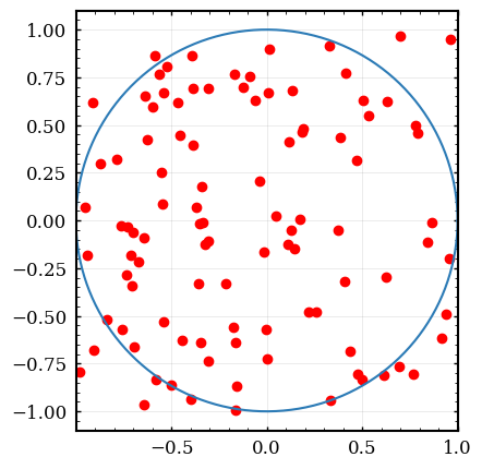
Monte Carlo simulation is a somewhat generic term used to describe repeated sampling (simulation) using random numbers as inputs. Lets explore a common example of Monte Carlo sampling: using a dart board to calculate the value of \(\pi\)
Imagine you have a dart board of radius 1m and can randomly throw darts at this board over the square range {-1m to 1m} in both the x and y directions. \(\pi\) can be calulated by “throwing” many darts uniformly over this range and counting the ones which land within r=1 of the center. Successful dart throws are used to calculate pi with the following ratios:
\[\text{ratio}=\frac{\text{inner}}{\text{total}} = \frac{\pi r^2}{\ell \cdot w} = \frac{\pi}{4}\]
\[\pi = 4\cdot \text{ratio}\]
The main advantage of the Monte Carlo method is how generic the application is to almost any problem. Simply create random numbers and let the computer hit the problem with a sledge hammer method. Much like a real sledge hammer, the Monte Carlo method is amazing at getting a job done quickly. Unfortunately sledge hammer methods are almost never the fastest at getting the job finished. Convergance for Monte Carlo is extremely slow. This negative property can be overcome with modern computers on simple problems. Specific sampling methods with much better convergance and more realistic properties exist in every field of science and engineering.
# Set up counters
inside=0
outside=0

guesses=100

for i in range(guesses):
  # use a random guess for x and y between -1 and 1
  guessx = random.rand()*2-1
  guessy = random.rand()*2-1

  if guessx**2+guessy**2<1:
    inside+=1
  else:
    outside+=1

  if i<500:
    plt.plot(guessx,guessy,'ro')

plt.plot(
      [numpy.cos(q) for q in numpy.arange(0,2*numpy.pi,0.01)],
      [numpy.sin(q) for q in numpy.arange(0,2*numpy.pi,0.01)])
plt.gca().set_aspect('equal')

print(guessx,guessy)
print("Inside: ",inside)
print("Outside: ",outside)
print("inside shots: ",inside/guesses*100,"% of area")
print("Pi: ",4*inside/guesses)

plt.savefig("img/02-dartboard.png",bbox_inches='tight')
plt.close()
#plt.show()
0.7011790903571216 0.9676352457448025
Inside:  84
Outside:  16
inside shots:  84.0 % of area
Pi:  3.36
Here is a smaller version of the above code, which excludes the figures:
# Compact version of Monte Carlo estimation of pi
guesses=1000000
inside=0
for i in range(guesses):
  if random.rand()**2+random.rand()**2<1:
    inside+=1
print(4*inside/guesses)
3.138804
3.2. Monte Carlo: Kinematics in 2D
Lets now use the Monte Carlo method to simulate our ball launch.
Simply using the kinematics equations and giving normally distributed random values for the initial height, initial velocity, and angle of incline.
from numpy.random import normal # import Gaussian RNG

# Declare measured initial conditions
yi, Eyi = 1, 0.002
vi, Evi = 4.6, 0.1
theta, Etheta = 30*numpy.pi/180, 1*numpy.pi/180
ay = -9.8027

# create a list of uniforly spaced numbers for the time axis
time=numpy.array(numpy.arange(0,1,0.01))

# perform the kinematics calculation a bunch o times
for i in range(100):
  # x=xi+vix*t = 0 + vi*sin(theta)*t
  xpath=normal(vi,Evi)*numpy.cos(normal(theta,Etheta))*time
  # y=yi+viy*t-4.9t^2 = yi + vi*sin(theta)*t-49.t^2
  ypath=normal(yi,Eyi)+normal(vi,Evi)*numpy.sin(normal(theta,Etheta))*time+0.5*ay*time**2

  plt.plot(xpath,ypath)

plt.ylim(0,1.4)
plt.xlabel('Horizontal Position (m)')
plt.ylabel('Vertical Position (m)')
plt.title('Projectile Motion')
plt.gca().set_aspect('equal')

plt.savefig("img/02-projectile.png",bbox_inches='tight')
plt.close()
#plt.show()
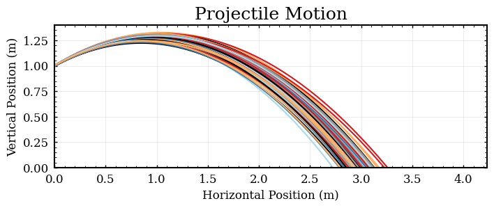
This is a very illustrative figure, but the code is not calculating what we want (you need an estimate of the horizontal range to report to the boss in an ’abstract’). The above code calculates x and y for a list of times (perfect for making a plot of the trajectories) but we want a distribution of horizontal ranges at a specific value of height. To proceed with the above data, you could search thru the list and find the list index (corresponding to a time) which the vertical position becomes negative. This sounds like a fine exercise for a programming assignment, but I wish to proceed in a different direction.
Instead, follow the standard method of calculating the range of an inclined shot from physics theory:
- Break up the velocity vector into components
- Use the y direction to solve for time (quadratic equation)
- Use the calculated time to find the range
Lets write a function to evaluate the solutions to the kinematic equations:
from numpy.random import normal # import Gaussian RNG
# vars to use as input: vi, theta, yi

# Step 1: vix=vi*cos(theta) viy=vi*sin(theta)
# Step 2: Kinematics in y-direction: 0=yi+vi*sin(theta)*t - 4.9 t^2
# this is a qadratic equation with a=-4.9 b=vi*sin(theta) c=yi
# t = (-b - sqrt(b*b - 4*a*c))/(2*a)
# Step 3: Kinematics x-direction: x = xi + vi*cos(q)*t

# requires 3 inputs: vi, theta, yi
# returns the calculated horizontal range
def ballistic_sim(vi,theta,yi):
  a,b,c=-4.9, vi*numpy.sin(theta), yi
  t = (-b - numpy.sqrt(b*b - 4*a*c))/(2*a)
  return vi*numpy.cos(theta)*t

# Calculate the trajectory for a randomly chosen set of input parameters
# uses numpy.random.normal() to generate random input values for vi, theta, and yi
for i in range(10):
  print("random shot",i,":",ballistic_sim(normal (vi,Evi),normal(theta,Etheta),normal(yi,Eyi)) )
random shot 0 : 2.8253864893107106
random shot 1 : 2.943230448713085
random shot 2 : 2.9486365004658768
random shot 3 : 2.942945481287842
random shot 4 : 3.0416240128377066
random shot 5 : 2.9694014633532553
random shot 6 : 2.889390480484175
random shot 7 : 2.8857552630417675
random shot 8 : 2.980195250559442
random shot 9 : 2.9117698534023706
shots=[ballistic_sim(normal(vi,Evi),normal(theta,Etheta),normal(yi,Eyi)) for i in range(50)]
print("Range: ",numpy.mean(shots),"+-", numpy.std(shots),"m")
plt.hist(shots,30)
plt.xlabel('Range (m)')
plt.ylabel('Frequency')
plt.title('Range Distribution')

plt.savefig("img/02-range.png",bbox_inches='tight')
plt.close()
#plt.show()
Range: 2.9589400681482583 +- 0.0942704914022101 m

Checkpoint:
- Make sure you can run the above code! (you must use your own data for the abstract)
- Propagate error for the initial velocity for the horizontal shot
- Record values for the angle and height (with measurement error)
- Use Monte Carlo to calculate the expected range for the inclined shot
4. Part 4: Writing an Abstract
Note: We are Math people. English is hard. Writing lab reports takes real effort and time. Writing an Abstract however, should only take you 10 or 15 minutes to complete.
To finish this lab exercise, you will practice writing an abstract. This is not a requirement for each lab, but is a critical skill for you to learn/hone in the future. This type of statement has 4 parts: Purpose, Method, Results, Conclusion (take a look at the link above more explanation).
Checkpoint:
- Write your abstract and submit!